Data Warehouse and BigQuery
OLAP vs OLTP
OLTP stands for ONline Transactions Processing, and OLAP stands for ONline Analytics Processing
OLTP is for backend purposes, while OLAP is used by data analysts or data scientists to discover insights.
| OLAP | OLTP | |
|---|---|---|
| Purpose | Control and run essential business operations in real time | Plan, solve problems, support decisions, discover hidden insights |
| Data updates | Short, fast updates initiated by the user | Data periodically refreshed with scheduled, long running batch jobs |
| Database design | Normalized databases for efficiency | Denormalized databases for analysis |
| Space requirements | Generally small if historical data is archived | Generally large due to aggregating large datasets |
| Backup and recovery | Regular Backups | Lost data can be recovered from OLTP insted of regular backups |
| Productivity | Increases productivity of end user | Increases productivity of managers and data analysts |
| Data view | Lists day-to-day business | Multi-dimensional view of enterprise data |
| User examples | Customer-facing personnel, clerks, online shopper | Knowledge workers and executives |
A data warehouse is a OLAP solution used for reporting and data analyses. It consists of raw data, metadata and summaries. They have many data sources.
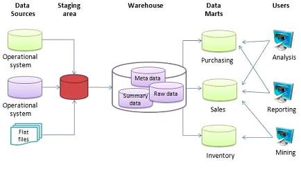
Data Warehouse can output to Data Marts (A data mart is a focused, smaller database containing a subset of data from a larger data warehouse, designed for a specific department (like Sales or Marketing) or business function, providing faster, easier access for targeted analysis, reporting, and business intelligence), but can also provide their raw output.
BigQuery
BigQuery is a serverless data warehouse. It provides both software and infrastructure, with scalability and availability in mind.
You can do ML via SQL, handle geospatial data and provide business intelligence solutions
BigQuery is flexible in how it handles data. BQ separates the compute engine that analyzes the data, from storage.
BQ has two pricing models:
- on demand pricing model; for every terabyte is $5
- flat price model based on number of pre requested slots; 100 slots -> $2000/month = 40TB data
BigQuery SQL Table Creation
1-- Query public available table
2SELECT station_id, name FROM
3    bigquery-public-data.new_york_citibike.citibike_stations
4LIMIT 100;1-- Creating external table referring to gcs path
2CREATE OR REPLACE EXTERNAL TABLE `taxi-rides-ny.nytaxi.external_yellow_tripdata`
3OPTIONS (
4 format = 'CSV',
5 uris = ['gs://nyc-tl-data/trip data/yellow_tripdata_2019-*.csv', 'gs://nyc-tl-data/trip data/yellow_tripdata_2020-*.csv']
6);When creating an external table (a table from an external resource), bq is not able to determine the size and number of rows
Partitioning
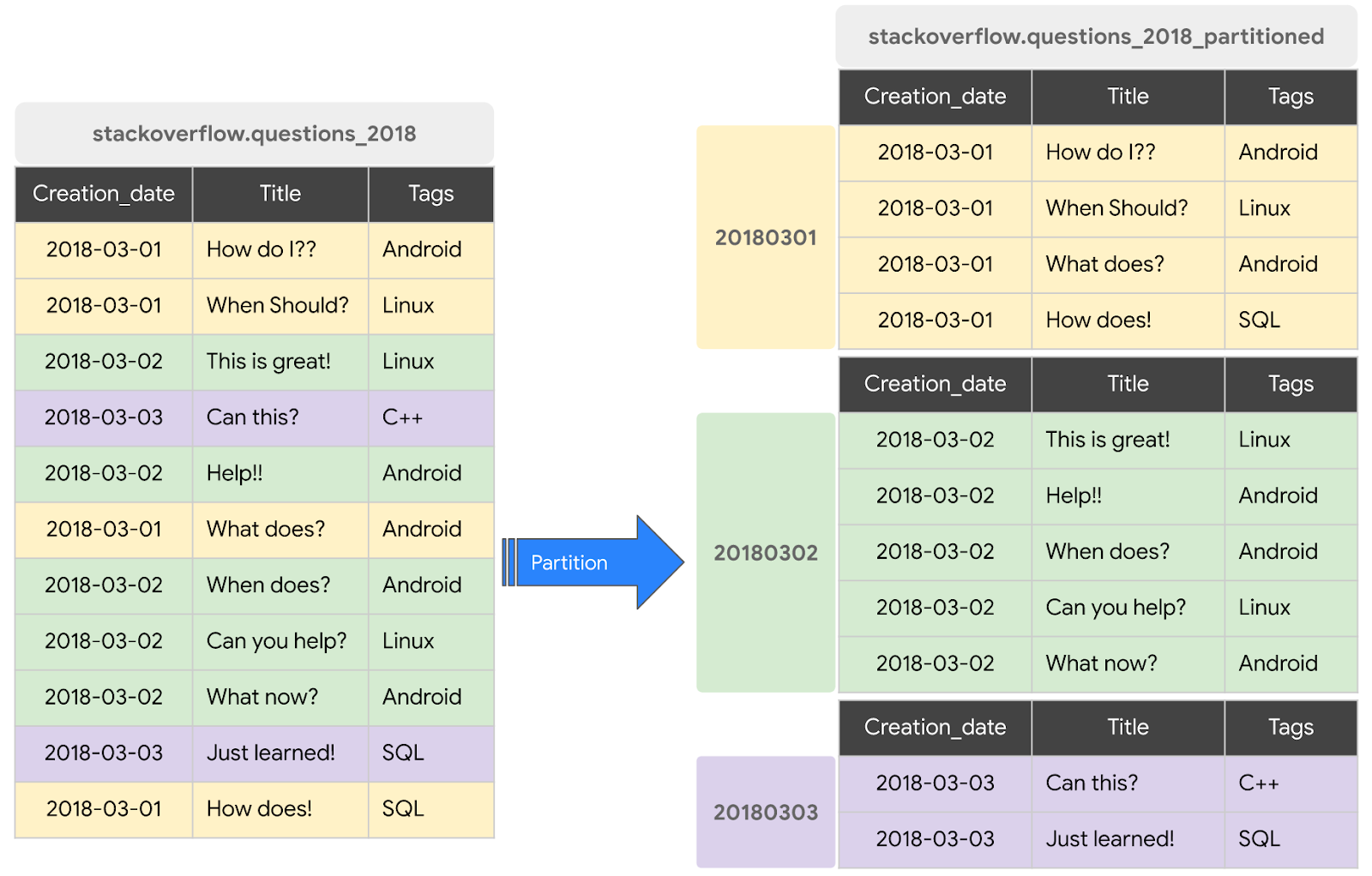
Generally when we create a dataset, we have columns, whose values can repeat. Partitioning can improve bq performance, by creating “buckets”, partitions of the raw dataset based on a columns value, like the date, improving cost and speed by processing less data upon runtime.
A partitioned table is divided into segments, called partitions, that make it easier to manage and query your data. By dividing a large table into smaller partitions, you can improve query performance and control costs by reducing the number of bytes read by a query. You partition tables by specifying a partition column which is used to segment the table.
 1-- Check yellow trip data
 2SELECT * FROM taxi-rides-ny.nytaxi.external_yellow_tripdata limit 10;
 3
 4-- Create a non partitioned table from external table
 5CREATE OR REPLACE TABLE taxi-rides-ny.nytaxi.yellow_tripdata_non_partitioned AS
 6SELECT * FROM taxi-rides-ny.nytaxi.external_yellow_tripdata;
 7
 8
 9-- Create a partitioned table from external table
10CREATE OR REPLACE TABLE taxi-rides-ny.nytaxi.yellow_tripdata_partitioned
11PARTITION BY
12  DATE(tpep_pickup_datetime) AS
13SELECT * FROM taxi-rides-ny.nytaxi.external_yellow_tripdata;
14
15-- Impact of partition
16-- Scanning 1.6GB of data
17SELECT DISTINCT(VendorID)
18FROM taxi-rides-ny.nytaxi.yellow_tripdata_non_partitioned
19WHERE DATE(tpep_pickup_datetime) BETWEEN '2019-06-01' AND '2019-06-30';
20
21-- Scanning ~106 MB of DATA
22SELECT DISTINCT(VendorID)
23FROM taxi-rides-ny.nytaxi.yellow_tripdata_partitioned
24WHERE DATE(tpep_pickup_datetime) BETWEEN '2019-06-01' AND '2019-06-30';
25
26-- Let's look into the partitions
27SELECT table_name, partition_id, total_rows
28FROM `nytaxi.INFORMATION_SCHEMA.PARTITIONS`
29WHERE table_name = 'yellow_tripdata_partitioned'
30ORDER BY total_rows DESC;
Clustering
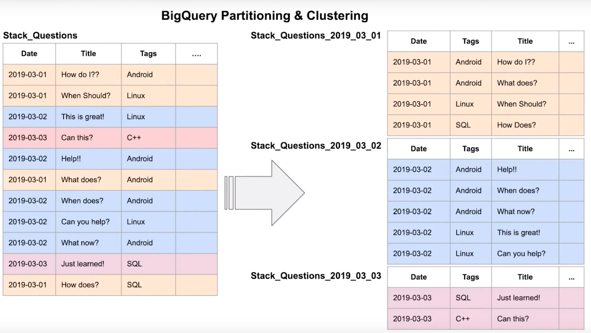
Clustered tables in BigQuery are tables that have a user-defined column sort order using clustered columns. Clustered tables can improve query performance and reduce query costs.
In BigQuery, a clustered column is a user-defined table property that sorts storage blocks based on the values in the clustered columns. The storage blocks are adaptively sized based on the size of the table.
When you create a clustered table in BigQuery, the table data is automatically organized based on the contents of one or more columns in the table’s schema. The columns you specify are used to colocate related data. When you cluster a table using multiple columns, the order of columns you specify is important. The order of the specified columns determines the sort order of the data.
 1-- Creating a partition and cluster table
 2CREATE OR REPLACE TABLE taxi-rides-ny.nytaxi.yellow_tripdata_partitioned_clustered
 3PARTITION BY DATE(tpep_pickup_datetime)
 4CLUSTER BY VendorID AS
 5SELECT * FROM taxi-rides-ny.nytaxi.external_yellow_tripdata;
 6
 7-- Query scans 1.1 GB
 8SELECT count(*) as trips
 9FROM taxi-rides-ny.nytaxi.yellow_tripdata_partitioned
10WHERE DATE(tpep_pickup_datetime) BETWEEN '2019-06-01' AND '2020-12-31'
11  AND VendorID=1;
12
13-- Query scans 864.5 MB
14SELECT count(*) as trips
15FROM taxi-rides-ny.nytaxi.yellow_tripdata_partitioned_clustered
16WHERE DATE(tpep_pickup_datetime) BETWEEN '2019-06-01' AND '2020-12-31'
17  AND VendorID=1;
Clustering vs Partitioning
When creating a partition table, you can choose to partition by time-unit column, ingestion time or integer-range partitioning. Number of partition limit is 4000.
When choosing time-unit or ingestion-time partitioning, you can select to partition by day (default), hour, month or year.
When clustering, the columns you specify are used to co-locate related data; the order of the column is important because it determines the sort order of the data. You can specify up to 4 clustering columns. The clustering columns must be top-level and non-repeating columns.
Clustering improves filter and aggregate queries.
It makes sense to have clustering or partitioning for data > 1GB; for tables smaller than 1GB, the overhead added by these can defeat the advantages.
| Clustering | Partitioning |
|---|---|
| Cost benefit unknown | Cost known upfront |
| You need more granularity than partitioning allows | You need partition-level management |
| Your queries commonly use filters or aggregation against multiple particular columns | Filter or aggregate on single column |
| The cardinality of the number of values in a column is large |
You would cluster instead of partition if:
- Partitioning results in a small amount of data per partition (approximately less than 1 GB)
- Partitioning results in a large number of partitions beyond the limits on partitioned tables
- Partitioning results in your mutation operations modifying the majority of partitions in the table frequently (for example, every few minutes)
Automatic Reclustering
As data is added to a clustered table:
- the newly inserted data can be written to blocks that contain key ranges that overlap with the key ranges in previously written blocks
- These overlapping keys weaken the sort property of the table
To maintain the performance characteristics of a clustered table:
- BigQuery performs automatic re-clustering in the background to restore the sort property of the table
- For partitioned tables, clustering is maintained for data within the scope of each partition.
- it is free
BigQuery Best Practices
- Cost Reduction
- Avoid
SELECT *: bq stores data in a columns storage, so specifying column name will save operation costs - Price the queries before running them
- Use clustered or partitioned tables
- Use streaming inserts with caution
- Materialize query results in stages
- Query Performance:
- Filter on partitioned columns
- Denormalizing data
- Use nested or repeated columns
- Use external data sources appropriately
- Don’t use it, in case u want a high query performance
- Reduce data before using a JOIN
- Do not treat WITH clauses as prepared statements
- Avoid oversharding tables
Internals of BigQuery
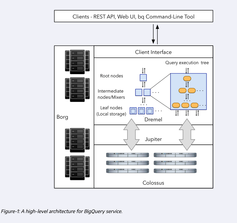
BigQuery stores the data in a separete storage called Colossus. It is a cheap storage that stores data in a column format. Since storage is separated from compute, it has significantly less cost. The most cost intensive task is reading the data itself, which is mostly compute.
Since compute and storage are on different hardware, how do they communicate? If network is bad, it can affect speed. That’s where Jupyter network playes a role. It is a network inside BQ datacenters, and provides 1TB/s network speed, allowing compute and storage to be on separated hardware while talking without any delays.
The third component of BQ is Dremel: it is bq execution engine; it divides queries into a tree structure, and separates queries in such a way that each tree node executes an individual subset of a query.
Columnar and Record-oriented storage
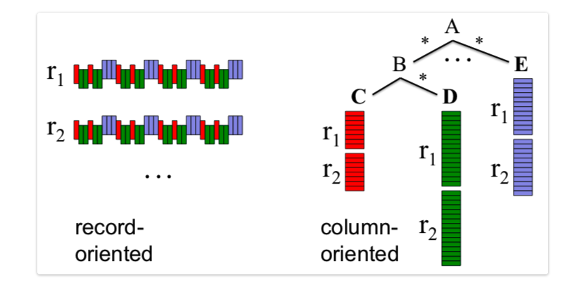
A record-oriented storage is the typical storage structure that we can find in CSV; each record (column) is their own entity, separated by a delimited (newline for CSV).
Column-oriented storage organizes data by column, storing all values for a single column together on disk, unlike traditional row-oriented systems that store all data for a single record sequentially. This method significantly speeds up analytical queries (like sums, averages, min/max) by allowing systems to read only the relevant columns, reducing I/O, and enabling efficient compression because data within a column is of the same type, making it ideal for data warehousing and big data analytics.
How it works:
- Data layout: Instead of
[Name1, Email1, Company1], [Name2, Email2, Company2], it stores[Name1, Name2, ...], [Email1, Email2, ...], [Company1, Company2, ...]. - Query optimization: For a query like “average sales amount”, the system only reads the “sales amount” column, ignoring others, which reduces data to process.
- Compression: Similar data types in a column (e.g., all numbers or all “Status: Active/Inactive”) compress much better, saving space and improving read speed.
- Vectorized processing: Storing data contiguously allows for modern CPU optimizations (like SIMD) to process chunks of data quickly,
Dremel
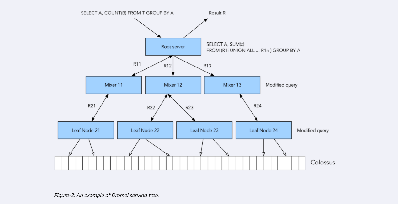
Dremel will modifiy the query that it receives into a number of subqueries that are delegated to mixers, which will further divide their own queries into subqueries until this process cannot be performed anymore, and the final subqueries are given to leaf nodes. These leaf nodes are the workers that will actually interface with Colossus to retrieve the data in parallel (MapReduce) and processes it and deliver it to the parent nodes until the original query is satisfied.
BigQuery ML
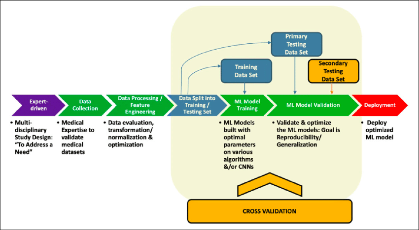
BQ helps in every step of the ML pipeline; it helps us do feature engineering, it can split data into training and evaluation, choose different algos, do hyperparameter tuning, it provides error matrices to do our evaluation, and it also allows us to deploy our model using Docker.
BQ has many different algorithms available depending on our scenario and use case. Let’s build a linear regression model against the ny-taxi data.
 1-- SELECT THE COLUMNS INTERESTED FOR YOU
 2SELECT passenger_count, trip_distance, PULocationID, DOLocationID, payment_type, fare_amount, tolls_amount, tip_amount
 3FROM `taxi-rides-ny.nytaxi.yellow_tripdata_partitioned` WHERE fare_amount != 0;
 4
 5-- CREATE A ML TABLE WITH APPROPRIATE TYPE
 6CREATE OR REPLACE TABLE `taxi-rides-ny.nytaxi.yellow_tripdata_ml` (
 7`passenger_count` INTEGER,
 8`trip_distance` FLOAT64,
 9`PULocationID` STRING,
10`DOLocationID` STRING,
11`payment_type` STRING,
12`fare_amount` FLOAT64,
13`tolls_amount` FLOAT64,
14`tip_amount` FLOAT64
15) AS (
16SELECT passenger_count, trip_distance, cast(PULocationID AS STRING), CAST(DOLocationID AS STRING),
17CAST(payment_type AS STRING), fare_amount, tolls_amount, tip_amount
18FROM `taxi-rides-ny.nytaxi.yellow_tripdata_partitioned` WHERE fare_amount != 0
19);
20
21-- CREATE MODEL WITH DEFAULT SETTING
22CREATE OR REPLACE MODEL `taxi-rides-ny.nytaxi.tip_model`
23OPTIONS
24(model_type='linear_reg',
25input_label_cols=['tip_amount'],
26DATA_SPLIT_METHOD='AUTO_SPLIT') AS
27SELECT
28*
29FROM
30`taxi-rides-ny.nytaxi.yellow_tripdata_ml`
31WHERE
32tip_amount IS NOT NULL;
33
34-- CHECK FEATURES
35SELECT * FROM ML.FEATURE_INFO(MODEL `taxi-rides-ny.nytaxi.tip_model`);
36
37-- EVALUATE THE MODEL
38SELECT
39*
40FROM
41ML.EVALUATE(MODEL `taxi-rides-ny.nytaxi.tip_model`,
42(
43SELECT
44*
45FROM
46`taxi-rides-ny.nytaxi.yellow_tripdata_ml`
47WHERE
48tip_amount IS NOT NULL
49));
50
51-- PREDICT THE MODEL
52SELECT
53*
54FROM
55ML.PREDICT(MODEL `taxi-rides-ny.nytaxi.tip_model`,
56(
57SELECT
58*
59FROM
60`taxi-rides-ny.nytaxi.yellow_tripdata_ml`
61WHERE
62tip_amount IS NOT NULL
63));
64
65-- PREDICT AND EXPLAIN
66SELECT
67*
68FROM
69ML.EXPLAIN_PREDICT(MODEL `taxi-rides-ny.nytaxi.tip_model`,
70(
71SELECT
72*
73FROM
74`taxi-rides-ny.nytaxi.yellow_tripdata_ml`
75WHERE
76tip_amount IS NOT NULL
77), STRUCT(3 as top_k_features));
78
79-- HYPER PARAM TUNNING
80CREATE OR REPLACE MODEL `taxi-rides-ny.nytaxi.tip_hyperparam_model`
81OPTIONS
82(model_type='linear_reg',
83input_label_cols=['tip_amount'],
84DATA_SPLIT_METHOD='AUTO_SPLIT',
85num_trials=5,
86max_parallel_trials=2,
87l1_reg=hparam_range(0, 20),
88l2_reg=hparam_candidates([0, 0.1, 1, 10])) AS
89SELECT
90*
91FROM
92`taxi-rides-ny.nytaxi.yellow_tripdata_ml`
93WHERE
94tip_amount IS NOT NULL;
Extract BQ Model and Deploy through Docker
Let’s authenticate through our CLI:
1gcloud auth loginSelect the project your model is on:
1gcloud config set project local-dimension-477102-g9Extract the ML model from BigQuery to a bucket:
1bq extract -m nytaxi.tip_model gs://nyc-tl-data-ld/tip_modelLet’s make a temporary folder where we will copy the model from the bucket to our local machine
1mkdir /tmp/model
2gsutil cp -r gs://nyc-tl-data-ld/tip_model /tmp/model
Let’s create a serving directory for model version 1, and copy the model in there
1mkdir -p serving_dir/tip_model/1
2cp -r /tmp/model/tip_model/* serving_dir/tip_model/1
Let’s now pull the docker image for serving and run it:
1docker pull tensorflow/serving
2docker run -d -p 8501:8501 --mount type=bind,source=`pwd`/serving_dir/tip_model,target=/models/tip_model -e MODEL_NAME=tip_model -t tensorflow/serving
Let’s query the model via http requests:
1curl http://localhost:8501/v1/models/tip_model
2
3curl -d '{"instances": [{"passenger_count":1, "trip_distance":12.2, "PULocationID":"193", "DOLocationID":"264", "payment_type":"2","fare_amount":20.4,"tolls_amount":0.0}]}' -X POST http://localhost:8501/v1/models/tip_model:predict
4`
#data-engineering #study-plan #career-development #zoomcamp #data marts